Home > Introduction > Tutorial > Build HAWT in DeepLines WIND tutorial
Build HAWT in DeepLines WIND tutorial
1. INTRODUCTION
This tutorial presents an example of a fixed horizontal axis wind turbine (HAWT) and its setup in DeepLines WIND as well as the results which can be post-processed.
A Blade Element Momentum (BEM) model is used to model the aerodynamics.Aerodynamic coefficients are used to calculate transverse and longitudinal forces on blades. Secondary effects such as Tip loss, Hub loss, Tower Shadow, Dynamic Stall, Skewed Effect, Dynamic inflow or 3D Effect can also be modelled but are not detailed in this document. Documentation on these cases can be found in Aerodeep 2.2 User Manual.
The fluid description (density and viscosity) can also be modified in the sea&ground panel. At the beginning of each time step, a) the mechanical solver provides information on positions, velocities, and accelerations at blades nodes as well as wind velocities data and b) the controller is called. The aerodynamic solver computes the resultant forces on each beam element. Within a time step, the aerodynamic forces are considered constant and are used to load the blades until convergence.
The example presented here is the NREL offshore 5MW baseline wind turbine with tower properties used for the OC4-DeepCwind semisubmersible. The model is shown below. This wind turbine is a conventional three-bladed upwind variable-speed variable blade-pitch-to-feather-controlled turbine.
The rotor blades are held by the hub. The hub rotates with the powertrain (shaft, gearbox and generator). The hub is initially clamped for static analysis then released for the dynamic phase. The nacelle is linked by 2 pin connections (acting as bearings) to the shaft. The nacelle is supported by the tower which is clamped at its bottom.
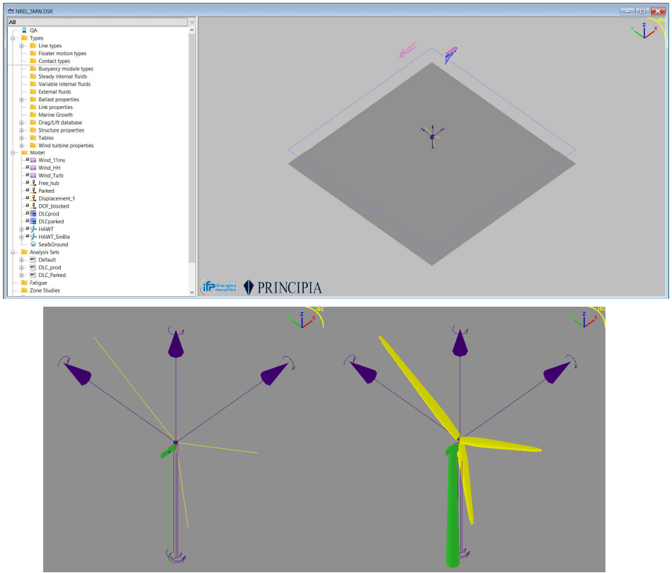
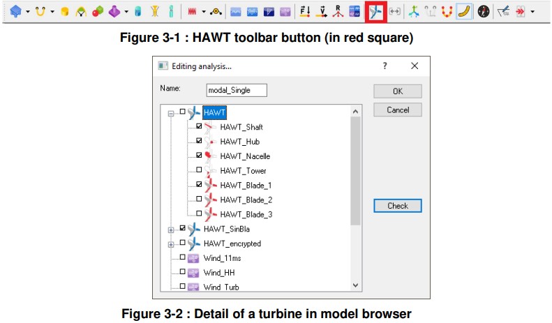
Figure 1-1 : Example of Wind turbine in DeepLines WIND
Table of Contents
1 INTRODUCTION
2 REFERENCES
3 BUILDING THE MODEL
3.1 MODEL COMPONENT: HAWT
3.1.1 General data
3.1.2 Turbine
3.1.3 Blades
3.1.4 Tower
3.1.5 Nacelle
3.1.6 Hub
3.1.7 Power train (shafts, gearbox, generator)
3.1.8 Control
3.1.9 Aerodynamic
3.2 MODEL COMPONENT: FREING THE HUB
3.3 MODEL COMPONENT: WIND
3.4 WIND TURBINE PROPERTIES
3.4.1 Control modes
3.4.2 Control dll options
3.4.3 Aero solver options
3.5 DRAG/LIFT DATABASE: FOIL PROFILES
3.6 ENVIRONMENT SET
4 STARTUP
4.1 SINGLE ANALYSIS
4.2 ANALYSIS SET
5 RESULTS
5.1 WIND, ROTOR AND GENERATOR
6 ANALYSES AND ANALYSIS SETS
6.1 RUNNING AN ANALYSIS
6.2 PROD_VR
6.3 PROD_VR_90
6.4 PROD_VR_HH
6.5 PROD_VR_TURB
6.6 PROD_VR_STARTUP_80S, 100S AND 120S
6.7 PROD_VR_STARTUP_X
6.8 PROD_VR_90_X
6.9 PROD_VR_90_X_1
6.10 PARKED_X
6.11 MODAL_GLOBAL
6.12 DLC_EXAMPLE
6.13 DLC_PARKED
6.14 DLC_EXAMPLE_STARTUP
7 APPENDIX: CONVENTIONS FOR HAWT
7.1 COORDINATE SYSTEMS FOR HAWT
7.2 PROFILE PROPERTIES
7.3 PITCH AND ATTACK ANGLE
7.4 COUPLING BETWEEN THE MECHANICAL AND AERODYNAMIC MODEL
7.5 TURBULENT WINDS
2. REFERENCES
| Ref. | Document Number | Document Title | Rev. |
|---|---|---|---|
| [1] | NREL/TP-500-38060 | Definition of a 5-MW Reference Wind Turbine for Offshore System Development | February 2009 |
| [2] | NREL/TP-5000-60601 | Definition of the Semisubmersible Floating System for Phase II of OC4 | September 2014 |
| [3] | - | Aerodeep 2.2 User Manual | Jan. 21 |
3. BUILDING THE MODEL
All orientations and conventions are provided in Section 7.
3.1. MODEL COMPONENT: HAWT
An HAWT is represented by lines and rigid bodies connected together. An HAWT is made of several subcomponents which are described in this section. HAWT subcomponents use a library named Aerodeep which includes a series of routine written to perform the aerodynamic calculations for aeroelastic simulations of the blades.
An HAWT is added to the model by clicking on the HAWT toolbar button (see Figure 3-1). This automatically created a shaft, a hub, a nacelle, a tower, and by default 3 blades (see Figure 3-2). The number of blades can be modified afterwards.
3.1.1. General data
General data are:
• The name of the turbine, if several turbines are modelled it is important to give them an appropriate name: it is called “HAWT” in this example.
• The position of the origin in the global coordinate system (when the turbine is free or clamped). This is the position of the bottom of the tower. Here it is 10 m above the MSL.
• The connection of the HAWT to other objects. In this example it is anchored and clamped which means that the bottom of the turbine does not move.
• The heading (generally not used, it is better practice to rotate the nacelle at the beginning of simulation.)
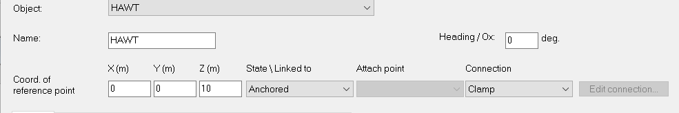
Figure 3-3 : Turbine general data
3.1.2. Turbine
This panel allows defining that the turbine is upwind, rotating clockwise and has 3 blades. The tower altitude is automatically updated with the tower length (see Tower sheet 3.1.4) and coordinates of reference point (see 3.1.1) and indicate that the top of the tower of 87.6m above the MSL. Several dimensions are defined as illustrated by the drawing provided in the sheet.
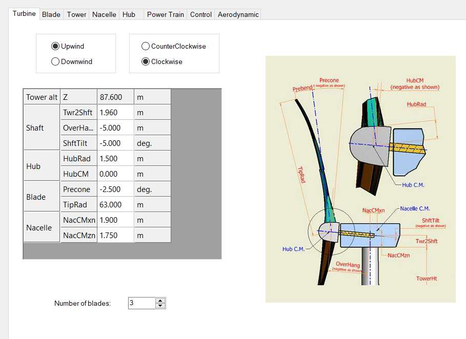
Figure 3-4 : Turbine general setup
3.1.3. Blades
Blades are modelled using beam finite elements. The “GENERIC” line type is used in DeepLines. Blades are clamped to the hub.
The shape and mechanical twist of the blades gives the equilibrium reference of the object (“User-defined shape”). The blade can be provided in an encrypted file or fully described. The shape of a fully described blade (which is the case here) is shown in the graphic interface and a visual check of the shape can be done (chord variations with length). The blade profiles are discussed in section 3.5. The 3 blades are similar and modifying values in the blade editor will modify the 3 blades.
In this example, no added mass is used for the blades. It would have been defined in a variation table otherwise and selected here. The blade is divided in 17 sections. A different line type is defined for each blade section. Sections are defined from hub to tip.
Data can be modified in the blade interface or in the line type interface:
• 17 sections are defined for the aerodynamic properties in NREL specification document [1],
• the structural properties are merged to correspond to these 17 sections. The total length of the blade (total of length of each section) must be consistent with the length defined in the turbine sheet (= TipRad – HubRad) otherwise an error message will appear.
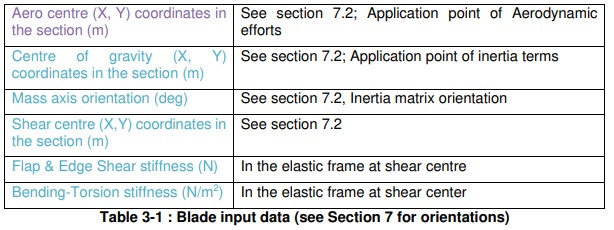
For each section, the following data should be provided. Data for structural and aerodynamic calculations are provided and are summarised in the table below.
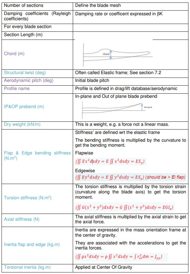
Blade orientation is shown in Figure 3-5. Z axis is positive from the hub to the blade tip.
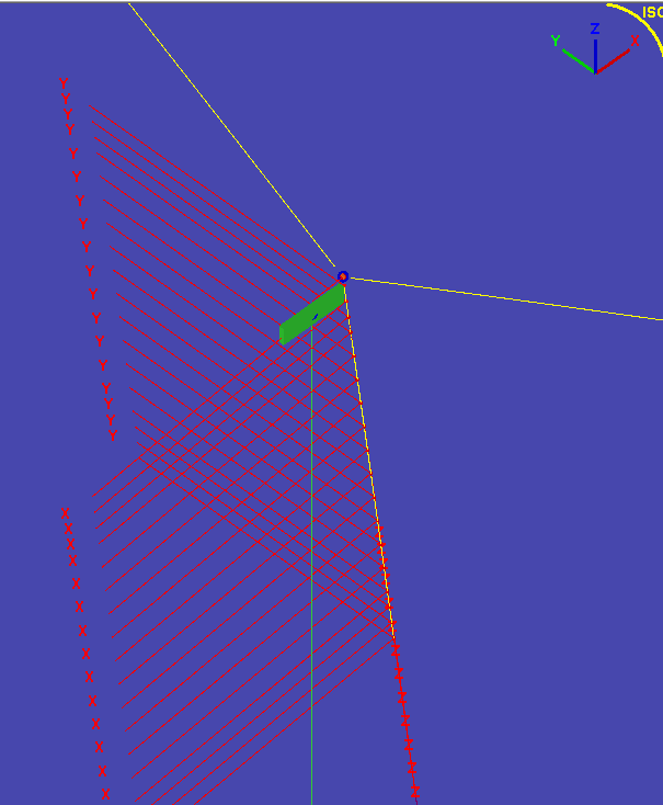
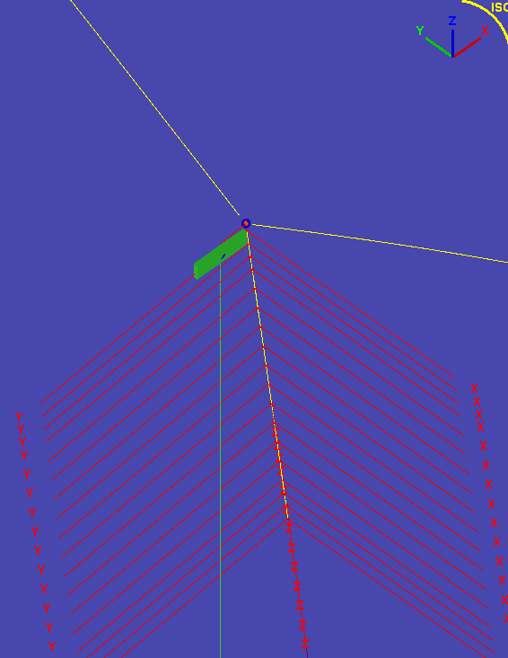
Figure 3-5 : Blade orientation. Top 0° (production), Bottom -90° (parked). Z is downwards here.
3.1.4 Tower
The tower is defined by beam elements.
The tower is clamped to the top at the Nacelle. The bottom of the tower can be anchored in space (which is the case in this example) or attached to another object (fairlead of a floater or rigid body).
A line type is automatically created with tower properties. The tower is a line divided in several segments. The number of segments is defined in “Partition”. A global drag coefficient can be defined on the tower and can depend on the Reynolds number. When defined, this drag coefficient supersedes the drag coefficients potentially defined in the segment types of the beam elements composing the tower.
This drag coefficient is used to apply wind load the tower. A specific drag coefficient is defined to compute the tower shadow which is only used by the aerodynamic solver. In this example a global drag coefficient of 0.65 is applied and is not depending on the Reynolds number.
Tower properties are the ones for the OC4-DeepCwind semisubmersible [2]. The tower length was set to 77.6 m. The tower type is conical. Therefore, the base diameter (6.5 m) and thickness (0.027 m), top diameter (3.87 m) and thickness (0.019 m) are input. The shape of the tower can be visually checked in the GUI.
The Young modulus, and specific gravity (= steel effective density/freshwater density) are also defined. A default value of Poisson coefficient equal to 0.3 has been chosen. A default value of Rayleigh damping coefficient of 0.005 has been chosen.
No drag coefficient for tower shadow is used in this example. See Aerodeep manual for more details [3].
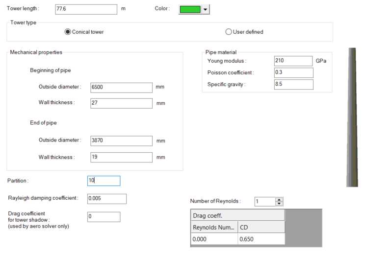
Figure 3-6 : Tower setup
3.1.5. Nacelle
The Nacelle is a rigid body in DeepLines.
• The tower is clamped to the Nacelle
• The shaft is linked to the Nacelle by pin connections
• The hub is clamped (to avoid convergence issue in static) and may be released using a displacement at the beginning of the dynamic simulation to allow the rotor to rotate (see Figure 3-15).
A box mesh is selected for viewing purposes.
Weight and rotational inertia can be specified, this is the case in this example.
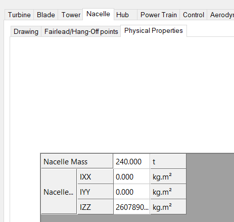
Figure 3-7 : Nacelle mass and inertia setup (see Section 7 for reference frame)
Polar wind coefficients can be added to the Nacelle, this is not the case in this example.
3.1.6. Hub
The hub is a rigid body in DeepLines
• The shaft is clamped to the Hub
• The blades are clamped to the Hub
A box mesh is selected for viewing purposes. Weight and rotational inertia can be specified, this is the case in this example.
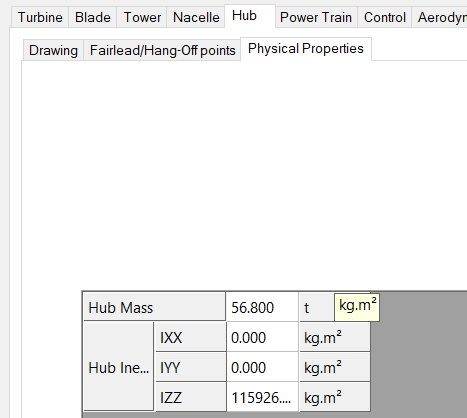
Figure 3-8 : Hub mass and inertia setup (see Section 7 for reference frame)
The reference frame is of the blades (to define twist/pitch) is shown by the hub “fairlead” points where the blades are clamped.
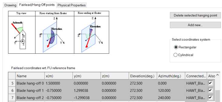
Figure 3-9 : Points of connection of the blades to the hub*
3.1.7. Power train (shafts, gearbox, generator)
The Shaft is composed of three beam elements.
Shaft properties are entered as a common line made of 3 segments (or 4 when HSS is used). A line type is created for the shaft. In this example, low speed shaft (LSS) properties only are specified. HSS is not used.
Default stiffness values are input to make the LSS highly rigid. Default lineic mass is input to make it nearly massless. Default Poisson coefficient value is chosen to make it not laterally expansible when compressed. Young modulus and specific gravity values are chosen considering the shaft is made of steel.
Outside diameter and wall thickness have generally no influence on the calculations when the mass is negligible and the thickness very high, which is very often the case.
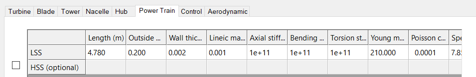
Figure 3-10 : Low speed shaft setup
A gear box ratio of 1/97 (<1) is input. This is the ratio between the rotor speed divided by the generator speed. Gearbox efficiency is taken equal to 1 (default value) meaning there is no power loss. The Gearbox ratio account for the multiplication factor between the high speed shaft and the low speed shaft.
The generator inertia is used in idling mode when the rotor is set free to rotate.
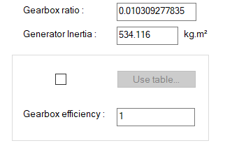
Figure 3-11 : Setup of generator and gearbox
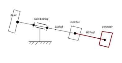
Figure 3-12 : Powertrain
3.1.8. Control
A dll is selected and a default mode is selected. See 3.4.1 and 3.4.2 for details on control modes and control dll options respectively. These are the default values, but they may be modified later on by using an EnvironmentSet (see 3.6). It is possible to edit the dll parameters by clicking on the “edit” button.
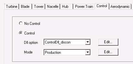
Figure 3-13 : Selection of control dll and mode
3.1.9. Aerodynamic
An aero solver is selected. See 3.4.3 for details on aero solver options. It is possible to edit the aero solver parameters by clicking on the “edit” button.
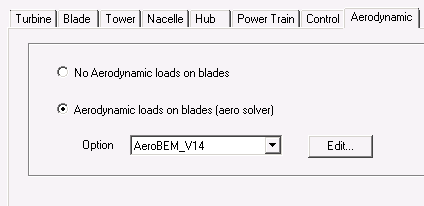
Figure 3-14 : Selection of aero solver
3.2. MODEL COMPONENT: FREING THE HUB
The hub needs to be freed at a beginning of a dynamic part of the simulation otherwise it will not rotate. A displacement (called Free_hub) of type Dis/connection has been added to the example which releases the HAWT COG. This displacement should then be added in the analyses.
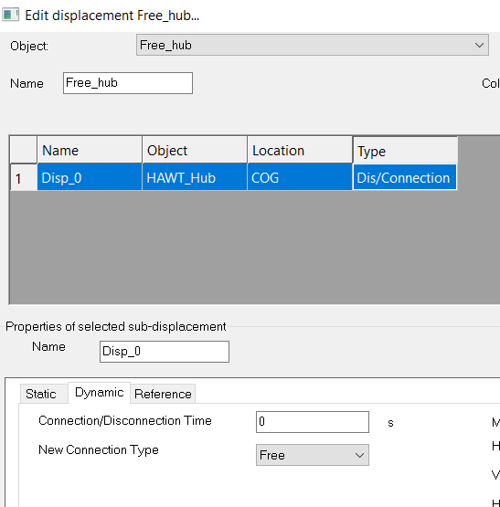
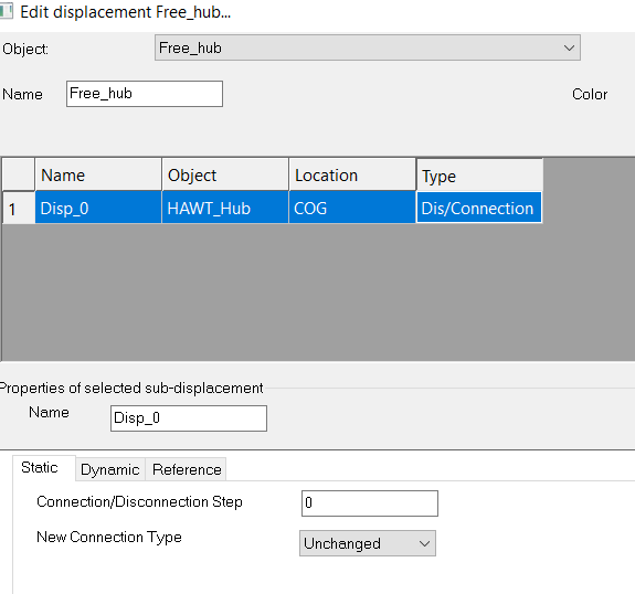
Figure 3-15 : Displacement used to release the rotor at the beginning of the dynamic simulation
3.3. MODEL COMPONENT: WIND
Different types of wind can be defined. Winds can also be modified in an EnvironmentSet (see 3.6).
This example used 3 different types of wind:
• Constant, called Wind_11ms. The heading and mean velocity are specified then the current speed is constant over height and time. A heading of 180° means that the wind is going towards X negative (DeepLines Global Frame). In this example the blades are facing the wind. This can be checked visually by selecting the wind and turbine in the interface.
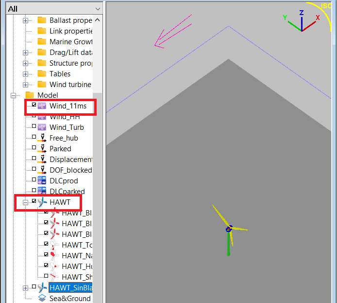
Figure 3-16 : Check of turbine and wind orientation with selection of wind and of turbine
• Time series of hub height wind (HH wind), called Wind_HH. The heading, the location of the wind file, the origin of the wind file wrt to DeepLines Global Frame and the width of the wind field should be specified. A width equal to 0 means the field is infinite. The example is simple, with only horizontal wind speed increasing with time, wind speed constant over height.
An example of wind file is shown below.
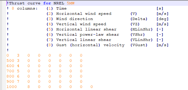
Figure 3-17 : HH wind file used in this example
• Time series of full field turbulent wind (FF wind), called Wind_Turb. The heading, the location of the .wnd wind file, the origin of the wind file wrt to DeepLines Global Frame, time for mirror effect, ramp time duration, beginning of turbulent wind should be specified. The .wnd file is an ASCII file.
Other types of wind are available but have not been used in this example.
3.4. WIND TURBINE PROPERTIES
3.4.1. Control modes
When defining a Turbine, four types of control can be performed:
• Blade Pitch (Displacement)
• Torque on the shaft for power generation (Force)
• Nacelle Yaw (Displacement)
• Brake on the Shaft (Force)
In the example, the generator and pitch control modes are selected in the Production Control Modes. The nacelle yaw control is not selected which means that the turbine is not dynamically controlled in yaw.
Note
Cut-in and cut-out wind speed are required but not used by the controller used in this example.
The generator-torque control requires the value of rated electric power, a torque rate limit, a minimum and maximum generated torque and generator efficiency.
Note
These values – except controller efficiency - are not used with the controller used in this example.
The blade-pitch control requires initial, minimum and maximum pitch values. The pitch control is here the same for the 3 blades (pitch control=collective) and the pitch type is the position.
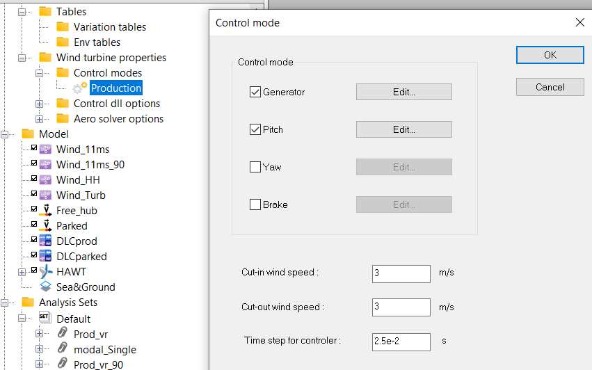
Figure 3-18 : Setup of control mode
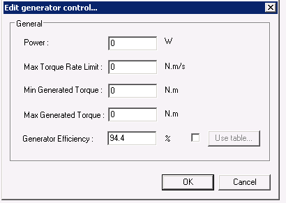
Figure 3-19 : Setup of generator control
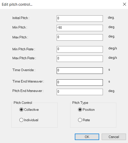
Figure 3-20 : Setup of pitch control
3.4.2. Control dll options
External dll are used to exchange information. In this example, control is applied on blade pitch and generator. The dll file and DLL procedure name have been specified. In this example (and this is often the case), the reference frame is defined by the mean wind direction.
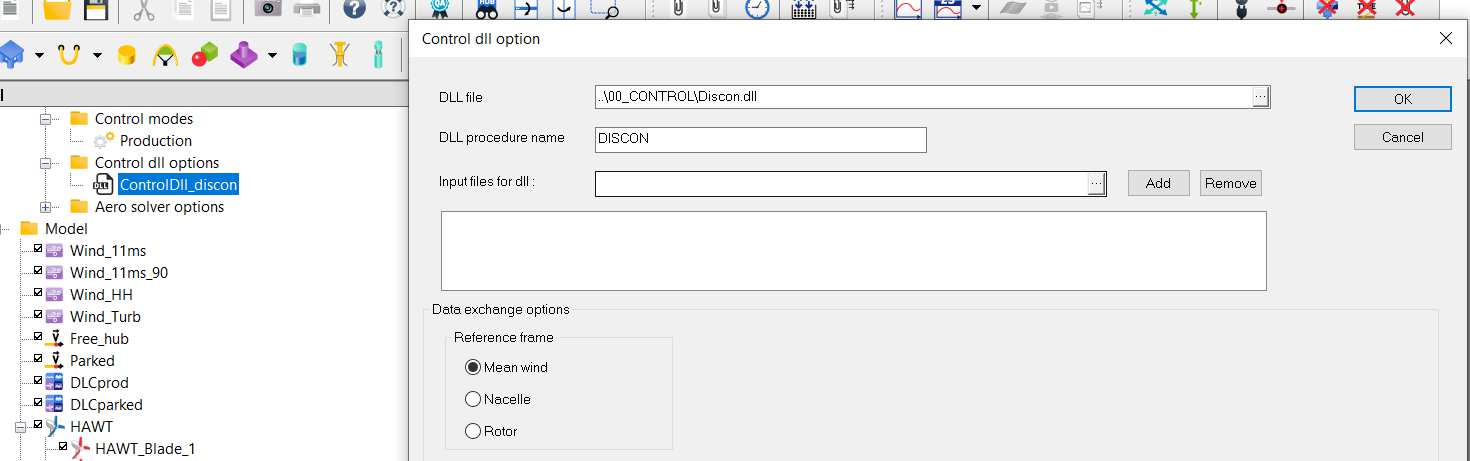
Figure 3-21 : Setup of control dll options
3.4.3. Aero solver options
An XML file for aerodynamic option could have been generated by ticking the available options. In this case, the .xml was already available and its location has been indicated. Blade profiles have been fully defined so there is no need to load an XML file for blade profiles.
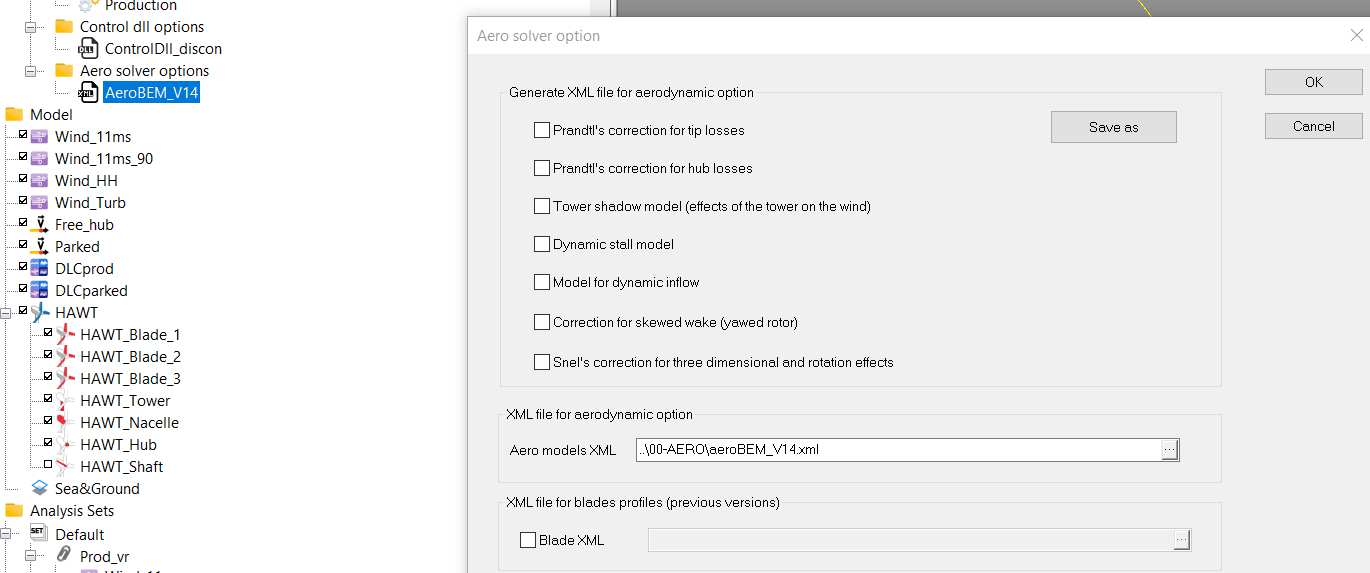
Figure 3-22 : Generation or selection of XML file for aerodynamic option and if necessary for blade profiles
3.5. DRAG/LIFT DATABASE: FOIL PROFILES
Each blade section is associated with a profile. Each profile type is defined in the drag/lift database. Values are not depending on Reynolds number in this example. The lift, drag and moment coefficients have been specified for attack angle between -180° and +180°. Attack angle is shown in Figure 3-24.
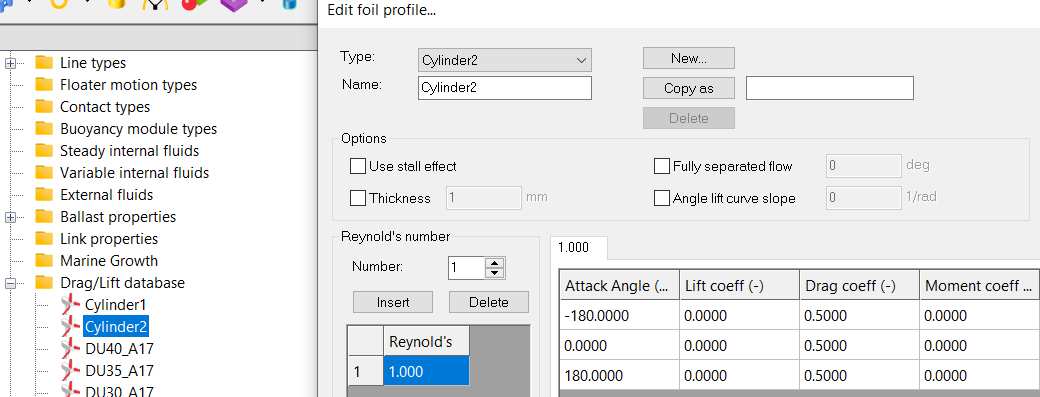
Figure 3-23 : Foil profile definition in drag/lift database
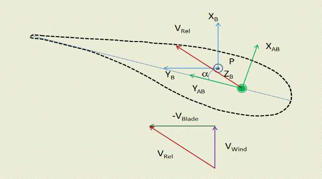
Figure 3-24 : Attack angle α: angle between incident flow and blade reference frame
3.6. ENVIRONMENT SET
Environment sets can be used to run an analysis set containing different wind files or control strategy.

Figure 3-25 : Environment set toolbar button (in red square)
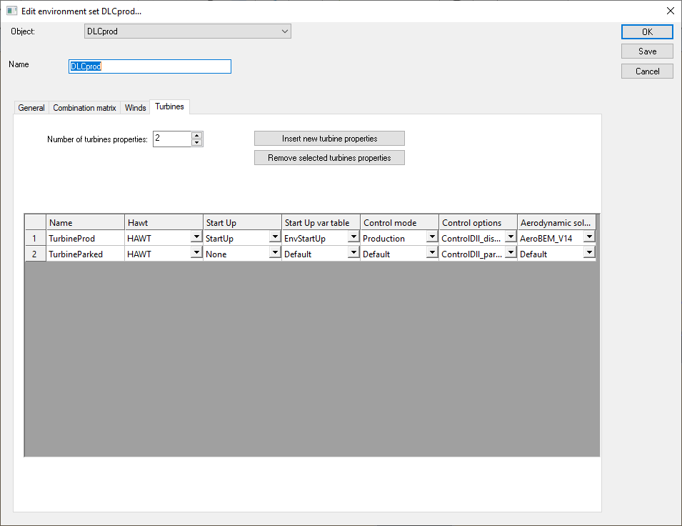
Figure 3-26 : Example of turbine options in an Environment Set
4. STARTUP
The startup of the turbine can be modelled using:
• a variation table (single analysis) and in addition for an analysis set an environment table which can be selected in the model browser (Figure 4-1),
• a displacement.
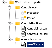
Figure 4-1 : Variation tables and environment tables in the model browser
4.1. SINGLE ANALYSIS
The variation table for start-up (Figure 4-2) should have 2 columns and at least 2 lines. The first one is filled with time (in s) and the second one with rotor velocity (in rad/s). In this example, the rotor velocity increases between 0 and -1.26 rad/s (=12 rpm) during the first 100s of the dynamic simulation. Velocity is negative to obtain a clockwise rotation of the rotor.
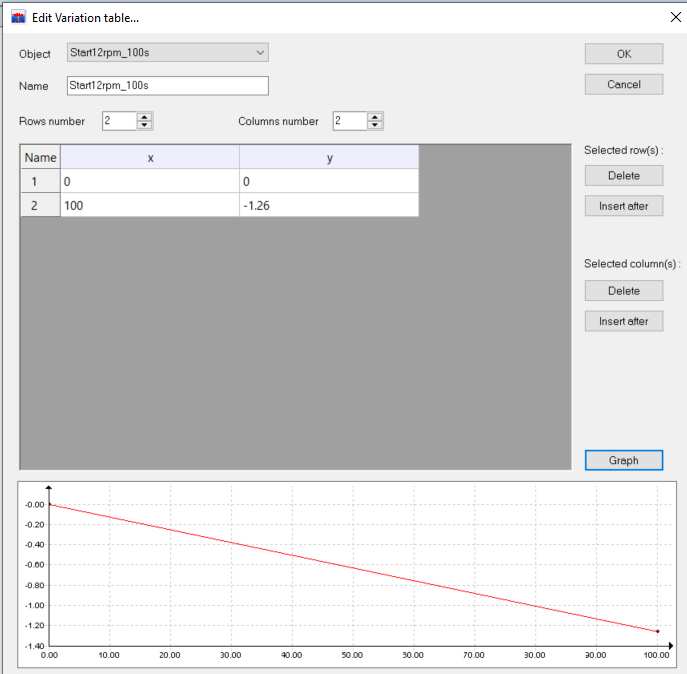
Figure 4-2: Example of variation table.
A displacement is used to impose the rotor velocity defined previously in the variation table. The displacement is imposed on the Hub and is of type “Control”. The type “Turbine start up” is selected in the relevant tab. The variation table is selected in the “prescribed speed” tab. ”End of start up” is used to specify at which time the startup control is released and the turbine control is taking over. This value should be taken into account when setting up the time in the variation table.
The displacement should be added in the analysis (see Figure 4-4). The analysis is ready to be run.
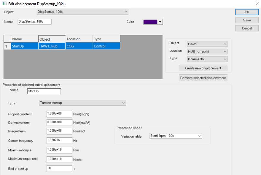
Figure 4-3: Displacement used to apply the variation table
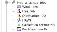
Figure 4-4: Displacement added in analysis
4.2 ANALYSIS SET
Startup can be done in an AnalysisSet with varying parameters depending on the analysis. The same setup than for a single analysis should be used. In addition, an environment table and environment set should be defined.
The environment table has 3 columns (see Figure 4-5).
• Index of the analysis in the analysis set. In this example, the first line corresponds to the last analysis of the analysis set. The environment table should have an index for each of the analysis in the analysis set. In this example there are 7 analyses in the analysis set. There should not be twice the same index in the first column of the environment table.
• Time in s. End of startup control time is the same for all the analysis in the environment set. So for example, for the 4th analysis in this analysis set, the rotor velocity of -1.26 rad/s is achieved at 80s then the turbine control starts at 100s. For the 5th analysis, a rotor velocity of approx. -1.26 rad/s is achieved at 100s then the turbine control starts (the velocity of -1.51 rad/s is not achieved).
• Rotor velocity in rad/s
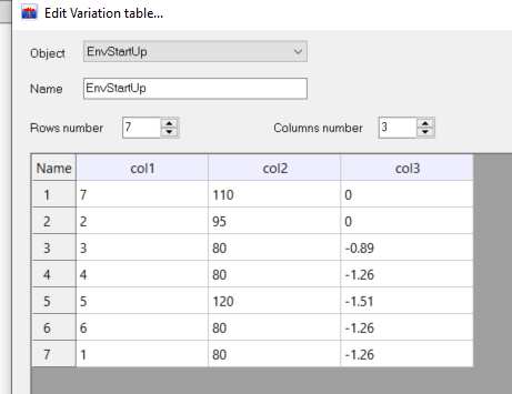
Figure 4-5: Environment table used in combination with environment set for turbine startup
An environment set is defined. In the turbine sheet:
• The turbine “HAWT” is selected
• The displacement “StartUp” is selected
• The environment table “EnvStartUp” is selected in the var table sheet
• Control mode, options and aerodynamics are selected to have the production behaviour of the turbine.
Then an analysis is created using this environment set.
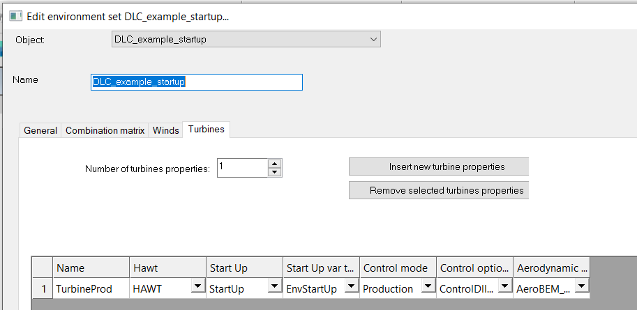
Figure 4-6: Environment set Turbine setup with startup
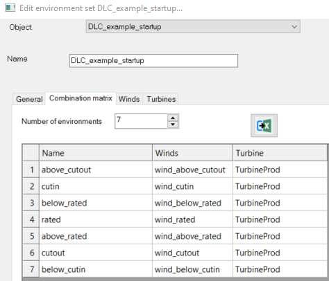
Figure 4-7: Environment set combination matrix with startup
5. RESULTS
Analyses are described in detail in the following section. The available results are presented in this section.
5.1. WIND, ROTOR AND GENERATOR
Specific turbine results can be accessed by selecting the Nacelle then diagnostics (see Figure 5-1). Data are also saved in the Turbine and Rotor files. In this example, these files are called turbine_HAWT.txt and rotor_HAWT.txt and are available in the analysis folder.
A list of specific turbine results is provided in table below. Attention must be paid to the units of the output results.
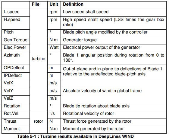
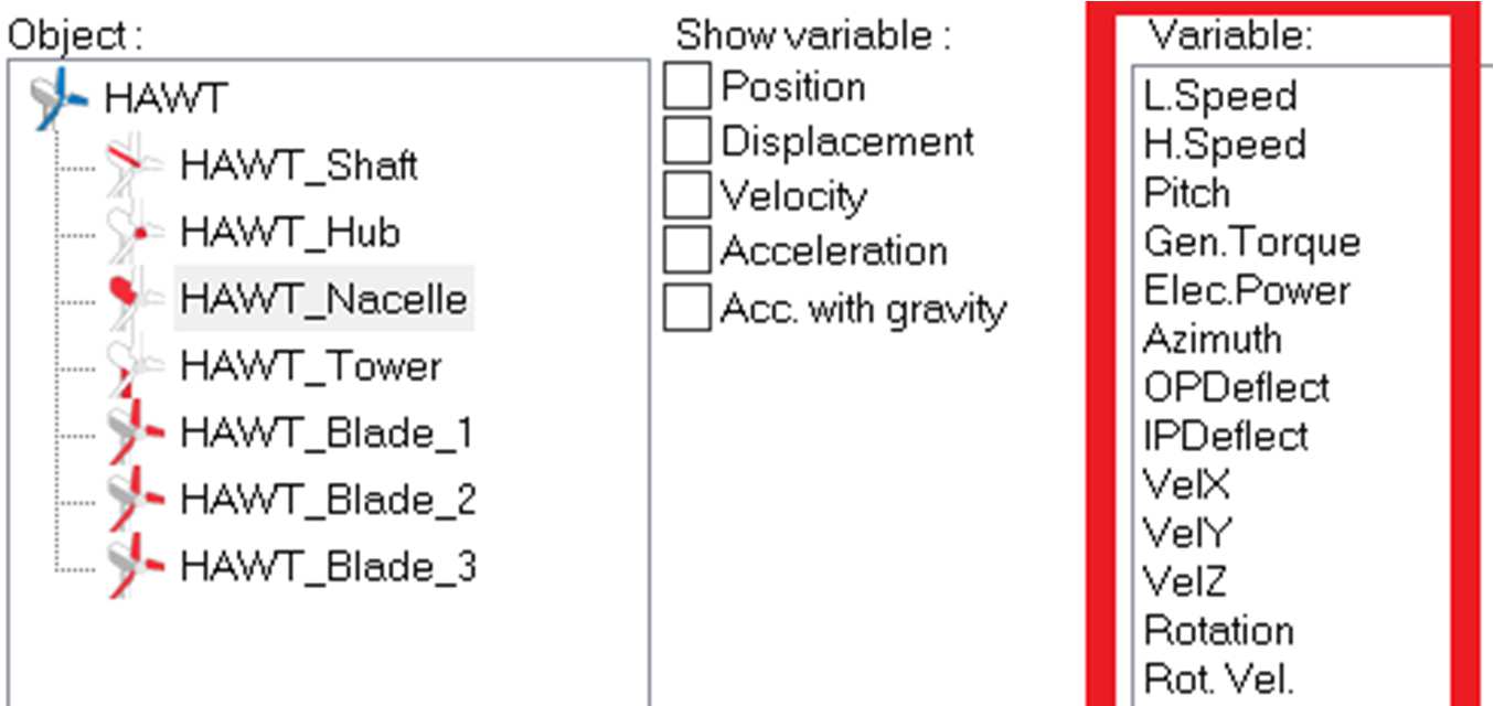
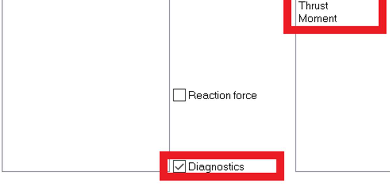
Figure 5-1 : Selection of turbine results
6. ANALYSES AND ANALYSIS SETS
6.1. RUNNING AN ANALYSIS
When the first analysis is run:
• Two JSON files named HAWT_1.JSON and HAWT_1_Blade.JSON are created into the AERO directory.
• HAWT.JSON contains data about the hub, the tower and the nacelle.
• HAWT_Blade.JSON contains data about the blades.
When an analysis is run, in addition to the typical analysis files, a turbine and a rotor files are created in the analysis folder.
6.2. PROD_VR
This simulation is run with a constant wind speed of 11.4 m/s (rated wind speed) (see VelX plot). The electrical power obtained once the turbine shows a steady behaviour. The electrical power is slightly below the rated power (5 MW).
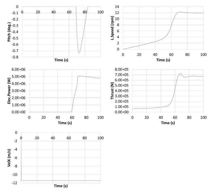
Figure 6-1 : PROD_VR results
6.3 PROD_VR_90
This is the same case than the previous one but the wind has been rotated by 90°. The turbine is rotated by 90° during the static calculation with the Displacement Yaw90. Results are similar to Prod_vr results.
6.4. PROD_VR_HH
This simulation is similar to prod_vr (6.2) but with a time series of wind instead of a constant wind.In this example, the wind speed is slowly increasing from 3 to 25 m/s. Wind is constant over height, without turbulence, and is facing the turbine.
Blade pitch angle varies during the simulation. The electrical power reaches its rated value when the wind speed (velX) reaches its rated value. The thrust increases until the wind speed reaches its rated value then the blade pitch angle changes and the thrust decreases.
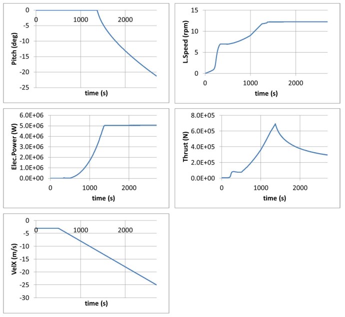
Figure 6-2 : PROD_VR_90 results
6.5. PROD_VR_TURB
This simulation is similar to prod_vr (5.2) but with a turbulent time series of wind instead of a constant wind. In this example, the wind speed is varying around the rated speed. Wind is constant over height and is facing the turbine. During the start of the turbine, the shaft speed, electrical power and thrust are increasing until stabilising (but still varying).
The blades could have pitched if required but this was not the case here.
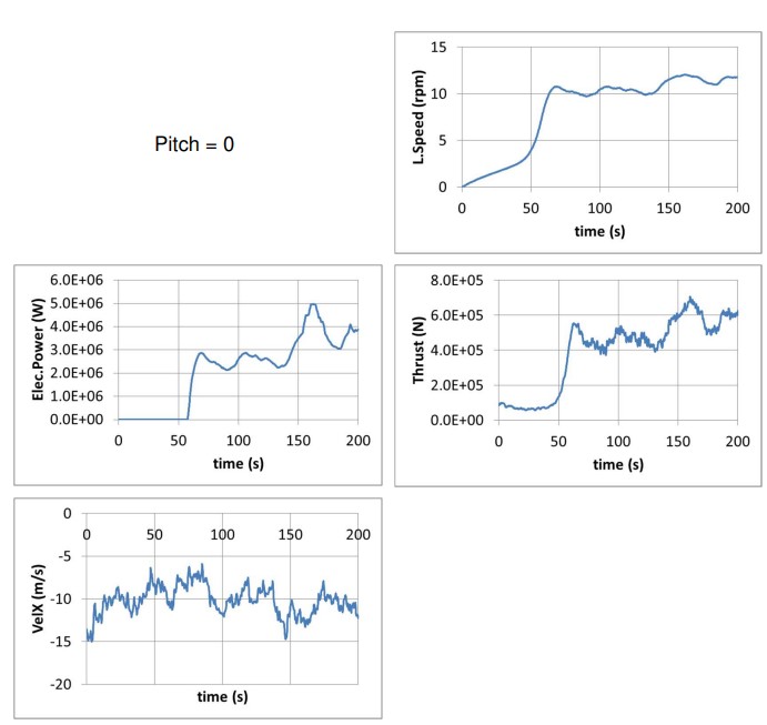
Figure 6-3 : PROD_VR_TURB results
6.6. PROD_VR_STARTUP_80S, 100S AND 120S
This simulation is run with a constant wind speed of 11 m/s slightly below the rated wind speed (11.4 m/s). Startup is applied in the variation tables during the first 80, 100 or 120 s of the simulation.
The variation table has 2 columns and at least 2 lines:
• First column: time in s
• Second column: rotation speed in rad/s. Please note the negative sign for a clockwise rotation.
A rotor speed of approx. 12 rpm should be achieved at 100 s in all cases, and even before (at 80s) for the 80s case. The startup control is turn off at 100s. Results are similar for the 100 and 120 s case.
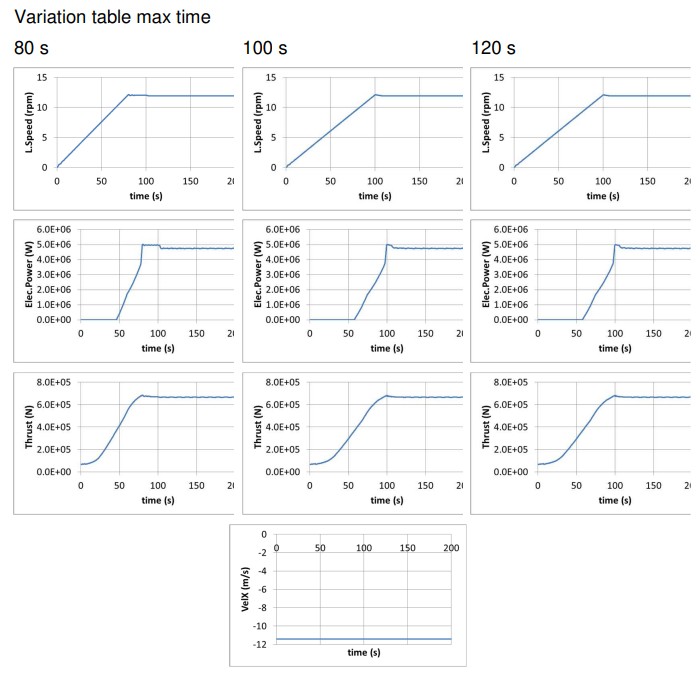
Figure 6-4 : PROD_VR_STARTUP_80S, 100S AND 120S results
6.7. PROD_VR_STARTUP_X
This simulation is the same than PROD_VR_STARTUP_100S but the setup is done in a different way, using a new feature. This new feature is particularly useful during the building and testing of the model.
In calculation parameters, the new sheet “HAWT properties” has been used and filled as follow:
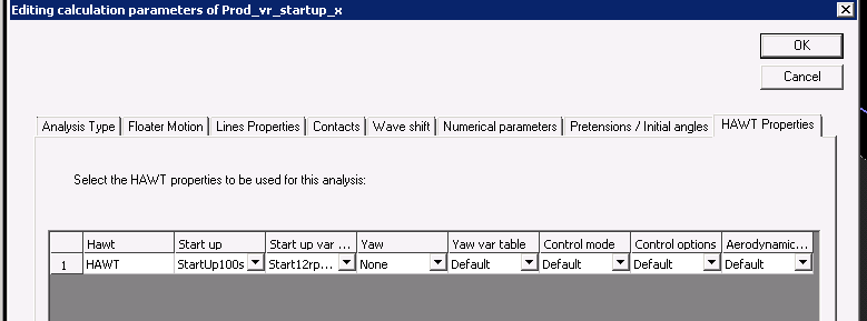
Figure 6-5 : Setup for startup in calculation parameters
Start up has been defined in a displacement and start up variable in a variation table as shown below. The start up variable could also have been set to “default” which would have automatically selected “Start12rpm_100s”.
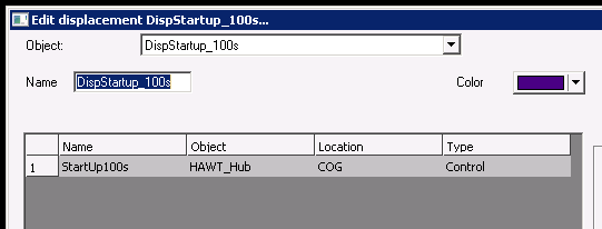
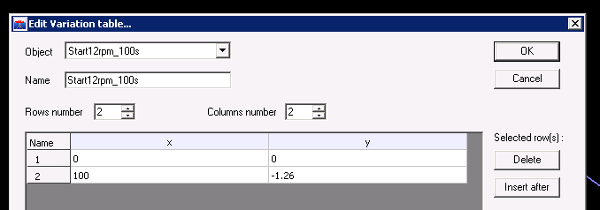
Figure 6-6 : Location of properties used in calculation parameters for startup
6.8 PROD_VR_90_X
This simulation is the same than PROD_VR_90 but the setup is done in a different way, using a new feature to rotate the turbine in yaw during static. This new feature is particularly useful during the building and testing of the model.
In calculation parameters, the new sheet “HAWT properties” has been used and filled as follow:
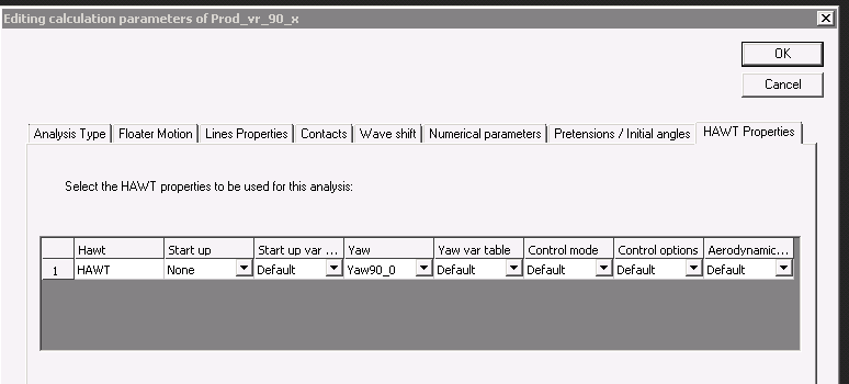
Figure 6-7 : Setup for initial yaw in calculation parameters
Yaw is defined in a displacement. The sub-displacement “Yaw90_0” is input in the setup showed above.
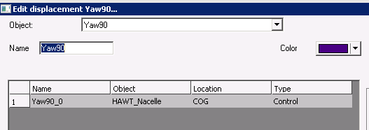
Figure 6-8 : Setup for initial yaw in calculation parameters
6.9. PROD_VR_90_X_1
This simulation is the same than PROD_VR_90 and PROD_VR_90_X but the setup is done in a different way, using a new feature, to rotate in yaw the turbine during static. This new feature is particularly useful during the building and testing of the model.
In calculation parameters, the new sheet “HAWT properties” has been used and filled as follow:
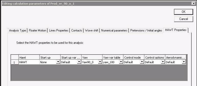
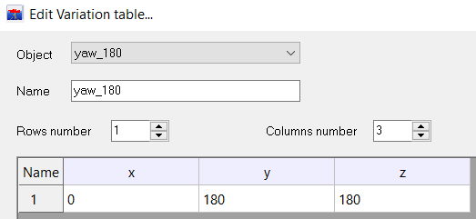
Figure 6-9 : Setup for rotation in yaw of the turbine during static in calculation parameters
The yaw variation table format should be 1 line with 3 columns:
• Initial step
• Final step
• Variation
In this case, results are similar than if the “yaw var table” parameter was using the default value, because 90 static steps are used. The yaw var table can be used to define different static angles.
6.10. PARKED_X
This simulation is the same than DLC_parked_parked, PROD_VR_90 or PROD_VR_90_X but the setup is done in a different way, using a new feature. This new feature is particularly useful during the building and testing of the model. In calculation parameters, the new sheet “HAWT properties” has been used and filled as follow:
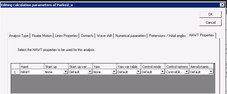
Figure 6-10 : Setup for parked in calculation parameters
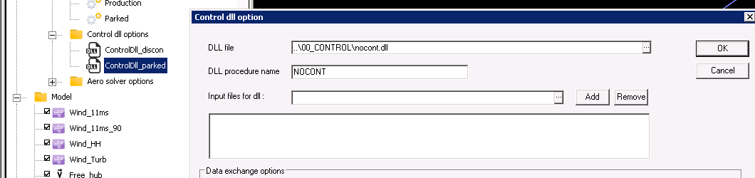
Figure 6-11 : Setup for control options in calculation parameters
6.11. MODAL_GLOBAL
This is a modal analysis with the whole turbine. Results are similar to typical modal analysis.

Figure 6-12 : View of dss of modal analysis
6.12. DLC_EXAMPLE
This is an analysis set with different production cases with wind speed varying from 2 to 30 m/s depending on the case. Wind speed is constant over time and height. A case (fixed) is also present in this analysis set for a case without control. However, the blades are not rotated by 90° to reduce thrust forces and therefore this is not a real parked case. See 6.13 for a parked case. Some results are shown below.
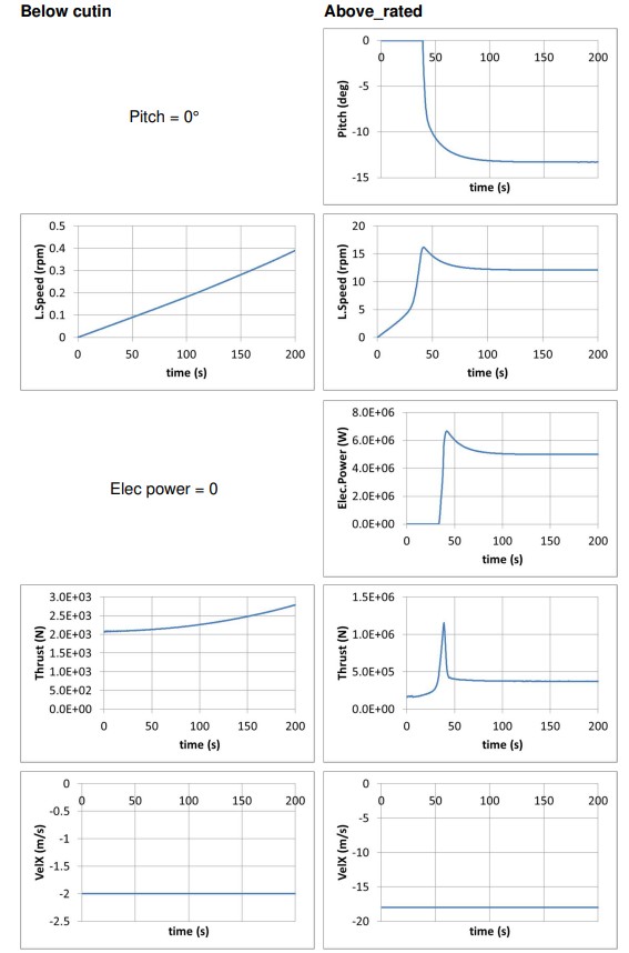
Figure 6-13 : DLC_example results
6.13. DLC_PARKED
The blades are rotated by a 90° angle during the static calculation in order to reduce the drag forces on them and consequently the thrust force. The hub is not released at the beginning of dynamic calculation. A dummy controller is used which does nothing. A DLC has been used to modify the parameter of the controller for this analysis only.
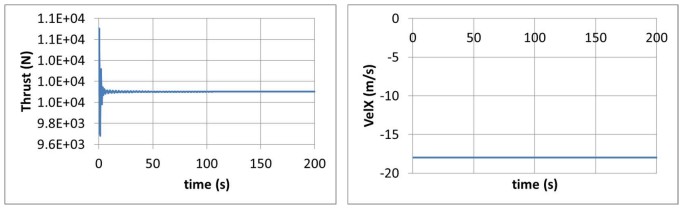
Figure 6-14 : DLC_parked results
6.14. DLC_EXAMPLE_STARTUP
This is an analysis set with different production cases with wind speed varying from 2 to 30 m/s depending on the case. Wind speed is constant over time and height. Startup is applied to all cases with different parameters.
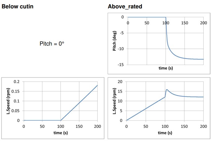
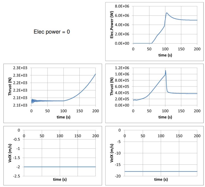
Figure 6-15 : DLC_example_startup results
7. APPENDIX: CONVENTIONS FOR HAWT
This section presents the conventions for HAWT.
7.1. COORDINATE SYSTEMS FOR HAWT
• Global coordinate system (G): DeepLines global coordinate system
o Origin: global frame origin
o XG: pointing to user required horizontal direction
o YG: (XG, YG, ZG) direct coordinate system
o ZG: pointing vertically upward opposite to gravity
• Nacelle coordinate system (N)
o Origin: rigid body reference point, top of the tower
o XN: defined by the heading of the turbine or by the heading (azimuth) of the fairlead point on which the turbine is connected
o YN: (XN, YN, ZN) direct coordinate system
o ZN: pointing vertically upward opposite to gravity
• Hub coordinate system (H)
o Origin: rigid body reference point; defined on the Nacelle as “Rotor Reference”
o XH: downward (shaft tilt from vertical direction)
o YH: (XH, YH, ZH) direct coordinate system
o ZH: hub rotation, upwind with shaft tilt from horizontal
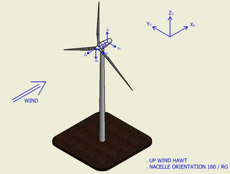
Figure 7-1 : Coordinate systems for HAWT: global, nacelle and hub
In the hub local frame, the blades initial pitch orientation is entered by the user. In most cases, it is defined in “production mode” where the pitch is close to 0° as opposed to the “feathered mode” where the pitch is close to -90°. In the following schematic, the blades are presented in production mode (No Tilt of the shaft).
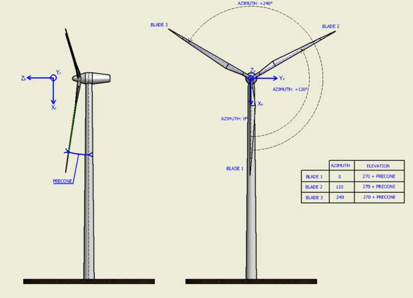
Figure 7-2 : Coordinate hub local frame
• Coned coordinate system (CO)
o Oriented by the blade fairleads of the hub
o XCO: in the (YH, ZH) plane
o YCO: (XCO, YCO, ZCO) direct coordinate system
o ZCO: in the blade axis at connection
The Coned coordinate system is represented below. This frame of reference is fixed with respect to the hub. Note that in the frame below, the blade is represented in feathered mode. The structural twist (elasticity), aerodynamic pitch (aerodynamics) and mass axis orientation (inertia) are defined in this frame.
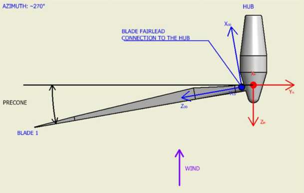
Figure 7-3 : Coned coordinate system
7.2. PROFILE PROPERTIES
A profile is defined by:
• A reference point P defined by the beam finite element in DeepLines (reference point of the Mechanical Blade coordinate system). The structural twist provides the rotation around the blade axis in the Blade coordinate system. Stiffness and inertia are defined in this reference system.
• The aerodynamic center position (x and y coordinate) and the CoG position (x and y coordinate) are defined in the Mechanical Blade (MB) frame (red frame below)
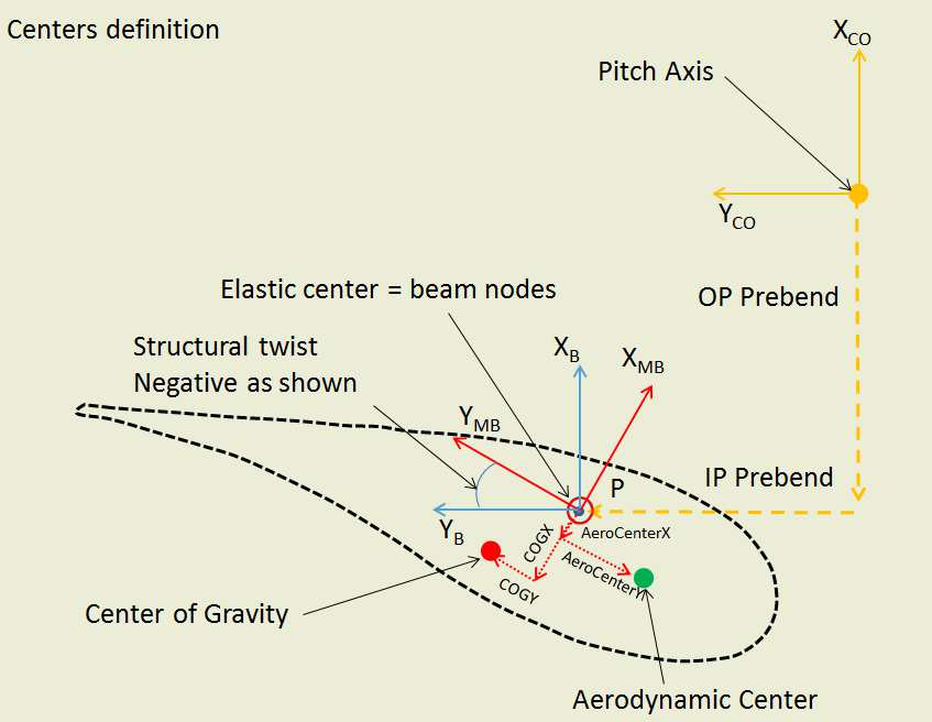
Figure 7-4 : Aerodynamic center position and COG in MB frame
• The aerodynamic pitch defines the direction for the aerodynamic loads (see section 6.3).
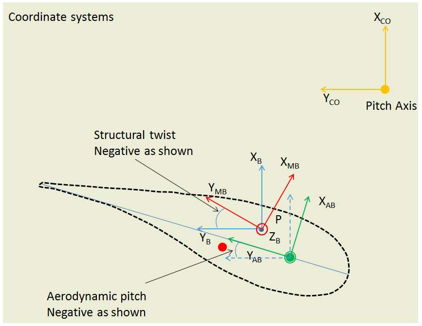
Figure 7-5 : Aerodynamic pitch
!!! Notes:
- The three nodes are at the same location unless COG and the AeroCenter locations are defined in the local frame of the blade section. To do so, their X and Y local coordinates shall be introduced (in meters) in the blade definition panel. <br>

- Mechanical stiffnesses are applied on the beam element point; no modification is introduced due to local (X, Y) coordinates of the COG. These local (X, Y) coordinates of the COG are used to calculate the moment due to the section weight to be applied on the beam point.
7.3. PITCH AND ATTACK ANGLE
The aerodynamic center is defined in the profile properties. The orientation of the Aerodynamic Blade frame may be different from the Mechanical Blade Frame. Therefore the aerodynamic pitch is defined for each section in the Blade coordinate system. If the aerodynamic pitch is equal to the structural twist, the Mechanical Blade and Aerodynamic Blade frames are the same.
• The Aerodynamic reference frame orientation is defined at the beginning of the calculations based on the aerodynamic pitch provided as input.
• An initial pitch may be added (see control definition panel > pitch > initial pitch);
• During the simulation, the pitch instruction from the controller is applied to the root of the blade and the blade torsion stiffness propagates it along the blade.
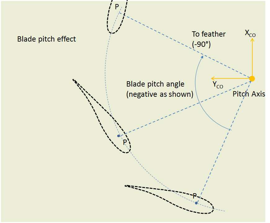
Figure 7-6 : Blade pitch angle
The combination of the wind speed and the local blade speed due to the turbine rotation generates an incident flow with an attack angle α with respect to the blade reference frame.
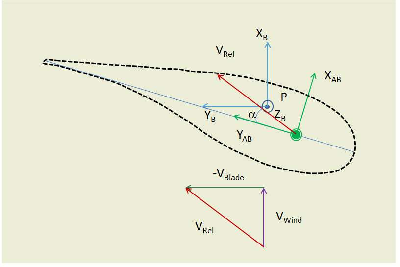
Figure 7-7 : Attack angle
The aerodynamic forces are derived from the attack angle and the polar coefficients associated with a profile.
7.4. COUPLING BETWEEN THE MECHANICAL AND AERODYNAMIC MODEL
All exchanges between DeepLines and the Aerodynamic solver are done in the global reference frame, which means at each time step:
DeepLines provides to the aerodynamic library the positions, the velocities, the wind speed as well as the blade local axes vectors in the global frame;
NB: These data are provided at the mechanical center P.
The aerodynamic library provides the aerodynamic forces and moments in the global frame. These efforts are derived from the attack angle, the relative velocities and the profile aerodynamic properties;
NB: The efforts are calculated at the Aerocenter.
In DeepLines, the local (X, Y) coordinates of the Aerocenter are used to derive the moment of the aerodynamic forces, calculated by the aerodynamic solver, to be applied on the beam point P. This moment is superimposed to the aerodynamic moment calculated with the Cm coefficient.
7.5. TURBULENT WINDS
Turbulent winds may be defined in specific files. At each time step, wind speeds are interpolated from the defined grids.
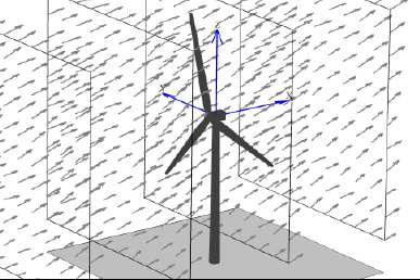
Figure 7-8 : Example of turbulent wind grid
These grids shall be previously generated with external software.
• The wind is defined by the keyword *WINDFILE (see keywords manual). A reference point as well as a heading angle may be defined to introduce the wind grids into the general DeepLines model in terms of (X,Y) and wind direction.
• These wind grids are fixed. They are not moving with the turbine. At each time step, the updated positions of any point of the model are used to interpolate the wind speed at that point.
